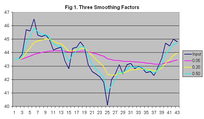
A number of different smoothing techniques can be used, such as moving averages and exponential weighted moving averages.

Smoothing Methods

The moving average method simply takes the average of the last x samples. The disadvantage of this is that you don't get a value until x samples have been read. Also, the averaged value tends to lag behind whenever the signal starts to change. An array could be used to store the samples. After filling the array, total the values of the samples and divide by the number of samples to get the average. Each time a new sample is received, it replaces the oldest sample in the array. Instead of having to re-total all samples again, just subtract the oldest sample from the total and add the new sample then divide the new total by the number of samples.

A more responsive method is called single exponential smoothing, or exponential weighted moving averaging (EWMA). Instead of treating each sample equally, samples are given exponentially decreasing weights as they get older so the newest samples are treated as most significant. A smoothing factor determines what percent of the smoothed value is calculated from the current sample with the remainder coming from the previous smoothed value. The user must choose the smoothing factor between 0 (0%) and 1 (100%) depending on how much the process varies and how smooth the result should be. Lower numbers give a smoother result because of more weight being given to past samples, while higher numbers cause it to more closely follow the current sample. In general, a useful smoothing factor is usually between 0.2 and 0.3. The actual exponential smoothing equation is:

SmoothedSample = (SmoothingFactor * CurrentSample) + ((1 - SmoothingFactor) * (LastSmoothedSample))

Note that for the first smoothed sample, there is no last smoothed sample to go by so the current input sample value has to be used.

Single exponential smoothing assumes the next value will be close to the last smoothed value. However, if the samples tend to follow increasing or decreasing trends, double exponential smoothing can be more effective. This method assumes the values will continue to follow the most recent rates of change. To calculate this, the rate of change (the difference between the current and last sample) is smoothed and added to the last smoothed sample. Now, there are two smoothing factors so the weight of previous values can be adjusted as well as how much to smooth the rate of change between each sample.

SmoothedSample = (SmoothingFactor * CurrentSample) + ((1 - SmoothingFactor) * (LastSmoothedSample + LastSmoothedChange))

SmoothedChange = (ChangeSmoothingFactor * (SmoothedSample - LastSmoothedSample)) + ((1 - ChangeSmoothingFactor) * LastSmoothedChange)

Note that for the first smoothed sample, there is no last smoothed sample to go by so the current input sample value has to be used. The first smoothed change value can be set to the difference between the current and next input samples. Other methods are available to calculate the initial value.

There is also triple exponential smoothing for samples which not only follow increasing or decreasing trends, but also have repeating patterns over time (seasonality). See the references below for more information.

Choosing The Smoothing Factors

The smoothing factor can be chosen through trial and error by trending the input value and smoothed value and observing the effect of different smoothing factors. Figure 1 shows a sample trend of an input value along with single exponential smoothing using three different smoothing factors. It is up to the user to decide the appropriate tradeoff between accuracy and smoothness.

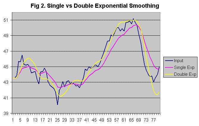
Figure 2 shows a sample trend of a process variable along with single and double exponential smoothing. The first 40 samples are fairly random and single smoothing works well. However, when the input value starts to consistently rise (samples 40 to 67) and fall (sample 67 to 77), single smoothing lags behind. Double exponential smoothing is able to follow the changes more closely, although it does overshoot when there is an abrupt change in the trend, as can be seen at sample 77.

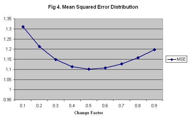
In figure 2, a smoothing factor of 0.20 and a change factor of 0.45 were used. The change factor was calculated using a simple method called least mean squared errors (MSE):

1. Find the error values (the difference between each input value and corresponding smoothed value) for a set of samples.
2. Square each error value and find the average. This is the MSE value.
3. Try this using different change factors for the same set of samples to find the change factor that results in the least MSE value.

Figure 3 demonstrates calculating the MSE for a small set of samples using double exponential smoothing with a smoothing factor of 0.1 and a change factor of 0.5 (normally, more samples should be used for a more accurate result).

Repeating the calculation with different change factors from .1 to .9 results in the following graph (figure 4). This shows that 0.5 is the optimal change smoothing factor value.

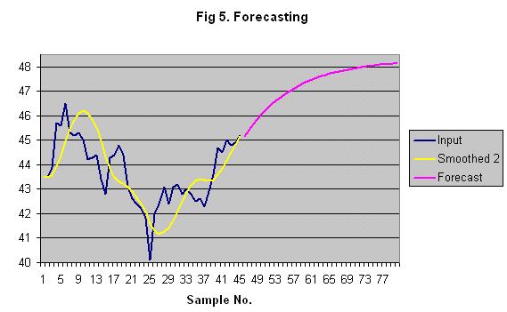
Forecasting

Double exponential smoothing can be used to predict future values, assuming the current upward or downward trend will continue. Just use the last smoothed sample in place of the current input sample in the calculations to predict the next input sample.

Cicode Smoothing Functions

The above equations could be used in a Cicode function to smooth a specific tag. Just substitute the input variable tag for CurrentSample and a disk variable tag for the SmoothedSample. The other values would need to be stored in Cicode variables until the next calculation. However this would mean creating a separate function and Cicode variables for each input tag. The attached Cicode file contains functions that can be used without modification for any number of input tags. Disk variable tags need to be created to hold the last values. The values of the variable tags as well as the tag names are passed to the functions. That way the function has the tag values without waiting for a TagRead(), and it can write the new values back to the variables with TagWrite(), which is non-blocking.

Label Name: Smooth(CurrSamp,SmFact,LastSmSamp,SampNo)
Label Expression: ExpSmooth(CurrSamp,SmFact,LastSmSamp,SampNo,#SampNo,#LastSmSamp)

Label Name: Smooth2(CurrSamp,SmFactor,LastSmSamp,ChgFactor,LastChgSamp,SampNo)
Label Expression: ExpSmooth2(CurrSamp,SmFactor,LastSmSamp,ChgFactor,LastChgSamp,#LastChgSamp,SampNo,#SampNo,#LastSmSamp)

References

NIST Engineering Statistics Handbook, http://www.itl.nist.gov/div898/handbook/pmc/section4/pmc43.htm
"Exponential Smoothing" by Philipp K. Janert, http://www.toyproblems.org/probs/p02/
"Exponential Smoothing", Wikipedia, http://en.wikipedia.org/wiki/Exponential_smoothing