Correlation chart calculations

Linear Regression Procedure (single response and multiple factors)

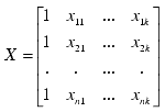
Simple Linear Regression is applied to fit a linear model of the form:

to continuous variables Y and X₁, X₂,...X_k.

Coefficients Estimation b₀, b₁,...b_k

Sum of squares of the residuals is:

where i is from 1 to n, n is the number of observations.

Estimation of b is done by the least square estimation; that is, minimizing the SS. By taking the derivative for each unknown b and setting each partial derivative to zero, k+1 linear equations are used to solve (k+1) unknown parameters.
X'X b = X'Y, where X' is the transpose matrix of X, and

Equations are solved by LU decomposition of X and then by forward-backward substitution.

Test Statistic Calculation

To test the Null Hypothesis H0:

vs. Alternative Hypothesis H1: at least one of them is non-zero.

where:

is the estimated coefficient, j = 0, ..., k.

is the mean of the y₁, y₂, y_n.

The sum of squares in the denominator above is called the Residual Sum of Squares (RSS), and the numerator of sum of squares is the Regression Sum of Squares.

P-Value Calculation

Test Statistic follows F Distribution with degrees of freedom (k-l, n-k).

Test Statistic and P-Values for each of the Correlation Coefficients

To test the null hypothesis estimated b _j = 0, the test statistic (T_j) is calculated with the following:

where:
is the j^th diagonal element of the dispersion matrix s2(X'X)^-1, and s² is the unbiased estimator of the variance, which is calculated as RSS/(n-k), and RSS is the residual sum of squares.

T_j follows Student's t distribution with (n-k) degrees of freedom.

Confidence Band - Confidence Interval (CI) Calculation

For each factor value (X), confidence interval is calculated (upper and lower Response values) using (1-a)% level of confidence, and plotted to get upper and lower bands.

where

MSR is Mean Residual Sum of Squares

SS_x is corrected Sum of Squares of X

t_a/2 = Student's t (n-2) value for a

Prediction Ellipse - Prediction Interval (PI) Calculation

The ellipse is determined based on the assumption that the two variables (X and Y) follow Bivariate Normal Distribution. The orientation of the ellipse is determined by the sign of the linear correlation between X and Y – the major axis of the ellipse is superimposed on the regression line. Probability (1-a) that a (X,Y) value will fall within the area that is marked by the ellipse is determined by the coefficient that defines the ellipse.

The ellipse coefficients are determined as follows:

Get the variance-covariance matrix between X and Y

It can be deduced that major and minor axes (l) of the ellipse are:

Data Plot Items

Scatter diagram of X values (Factor) and Y values (Response)
Linear Regression line (Y = aX + b)
Confidence Bands
Prediction Ellipse